Generate tedana walkthrough figures#
Important
The contents of this chapter will be moved into TE_Dependence and, to a lesser extent, Signal_Decay, and this chapter will be removed.
Load data#
Echo-specific timeseries#
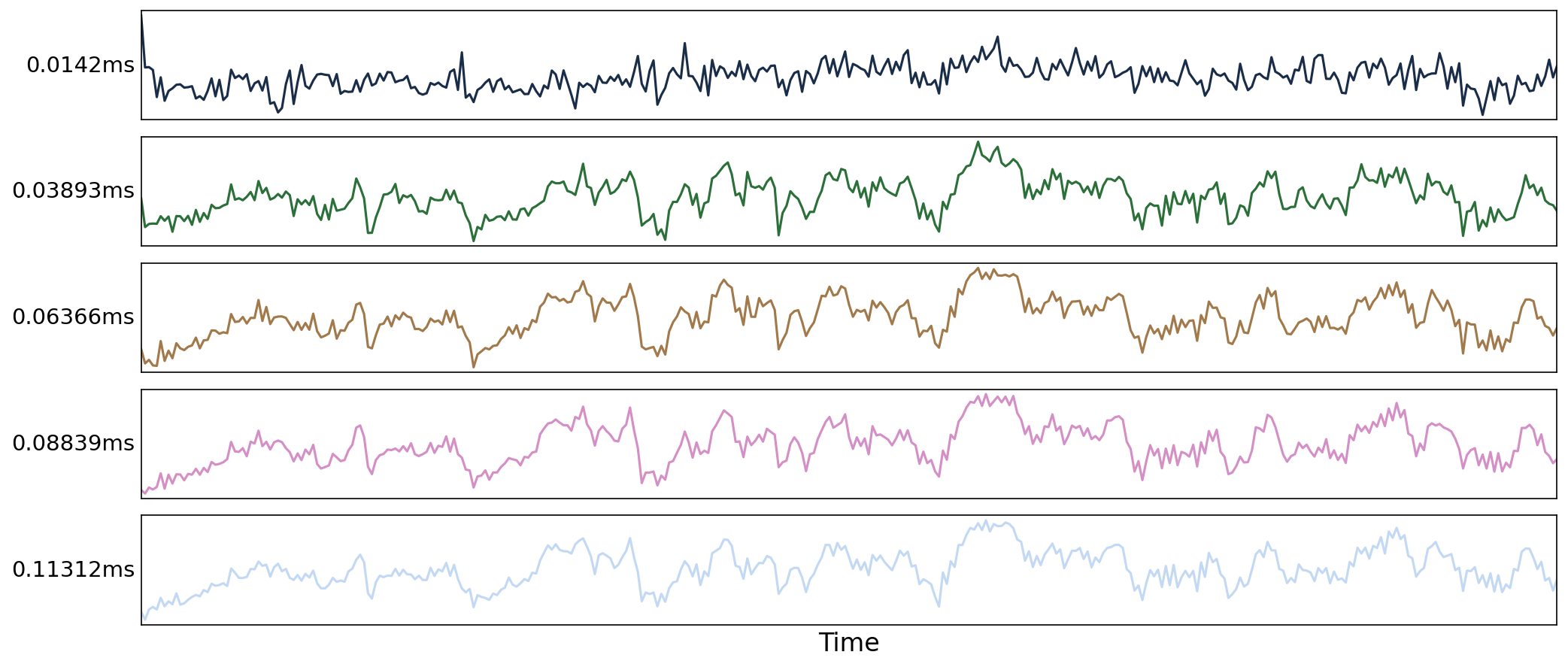
Fig. 22 Time series from a voxel for each echo.#
Echo-specific data and echo time#
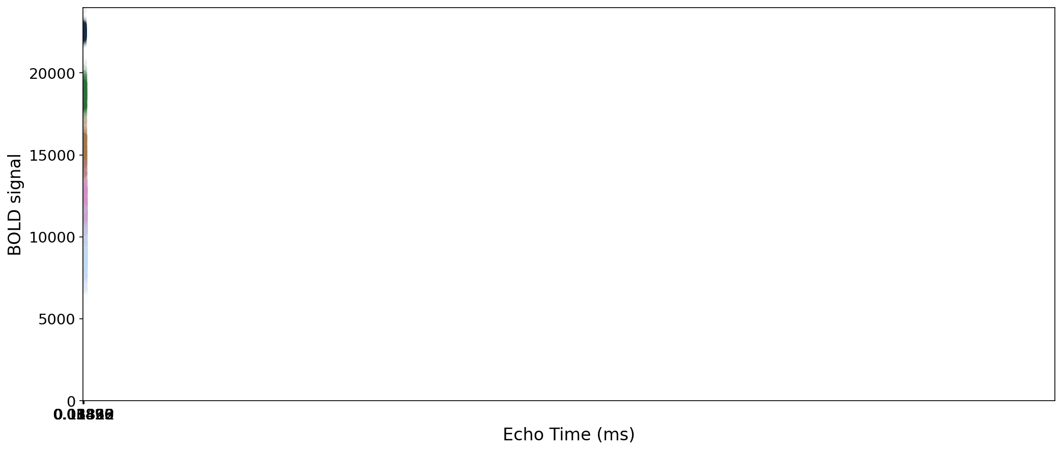
Fig. 23 Scatter plot of voxel’s values by echo time.#
Adaptive mask#
Longer echo times are more susceptible to signal dropout, which means that certain brain regions
(e.g., orbitofrontal cortex, temporal poles) will only have good signal for some echoes.
In order to avoid using bad signal from affected echoes in calculating \(T_{2}^*\) and \(S_{0}\) for a given voxel,
tedana generates an adaptive mask, where the value for each voxel is the number of echoes with “good” signal.
When \(T_{2}^*\) and \(S_{0}\) are calculated below, each voxel’s values are only calculated from the first \(n\) echoes,
where \(n\) is the value for that voxel in the adaptive mask.
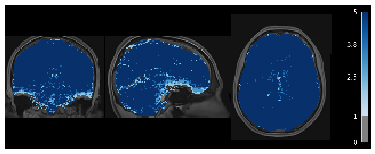
Fig. 24 Adaptive mask.#
Log-linear transformation#
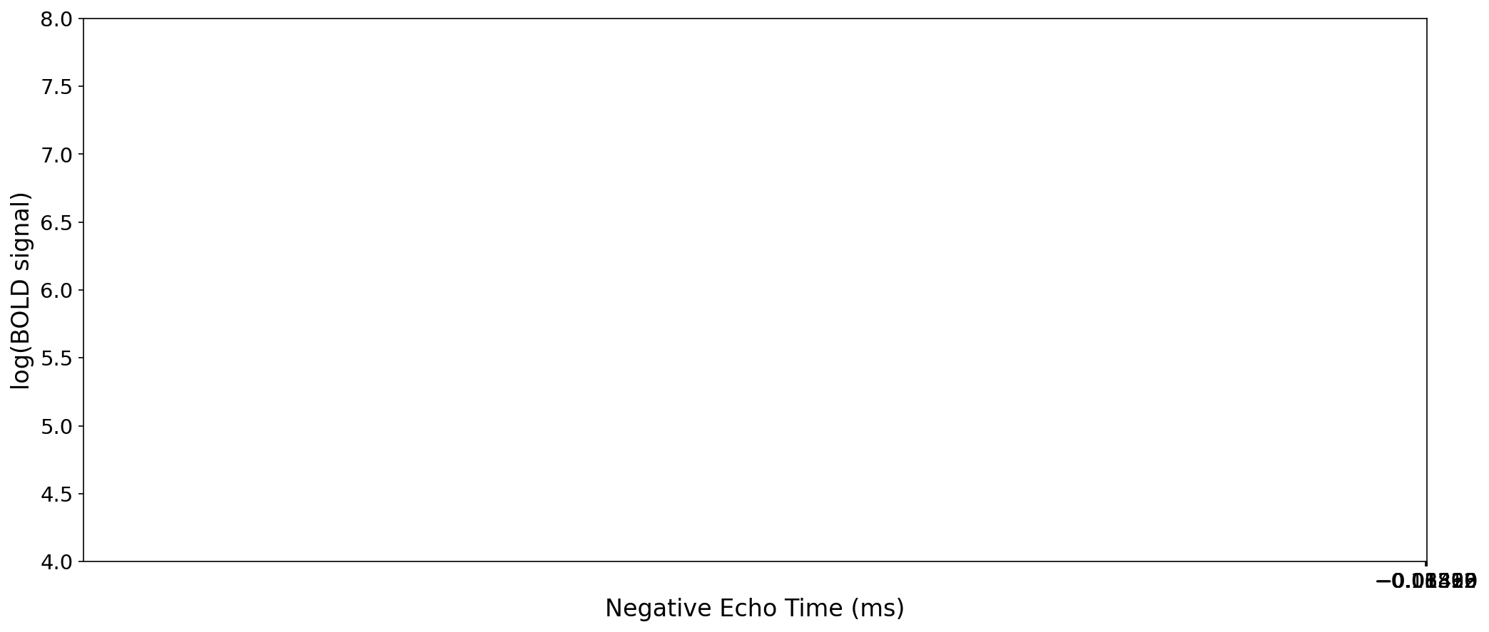
Fig. 25 Scatter plot of voxel’s signal for each echo, after log-linear transformation.#
Log-linear model#
Let \(S\) be the BOLD signal for a given echo.
Let \(TE\) be the echo time in milliseconds.
Fig. 26 Scatter plot of voxel’s signal for each echo, after log-linear transformation, with fitted line.#
Monoexponential decay model#
Calculation of \(S_{0}\) and \(T_{2}^{*}\)
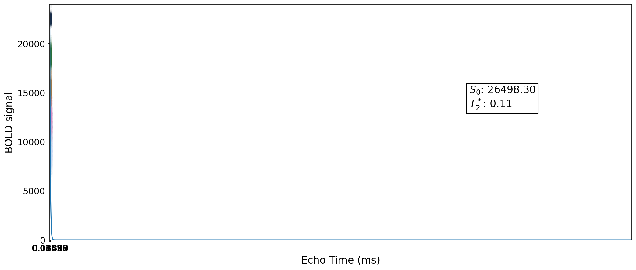
Fig. 27 Scatter plot of voxel’s signal for each echo, after log-linear transformation, with fitted line and T2* estimate.#
T2*#
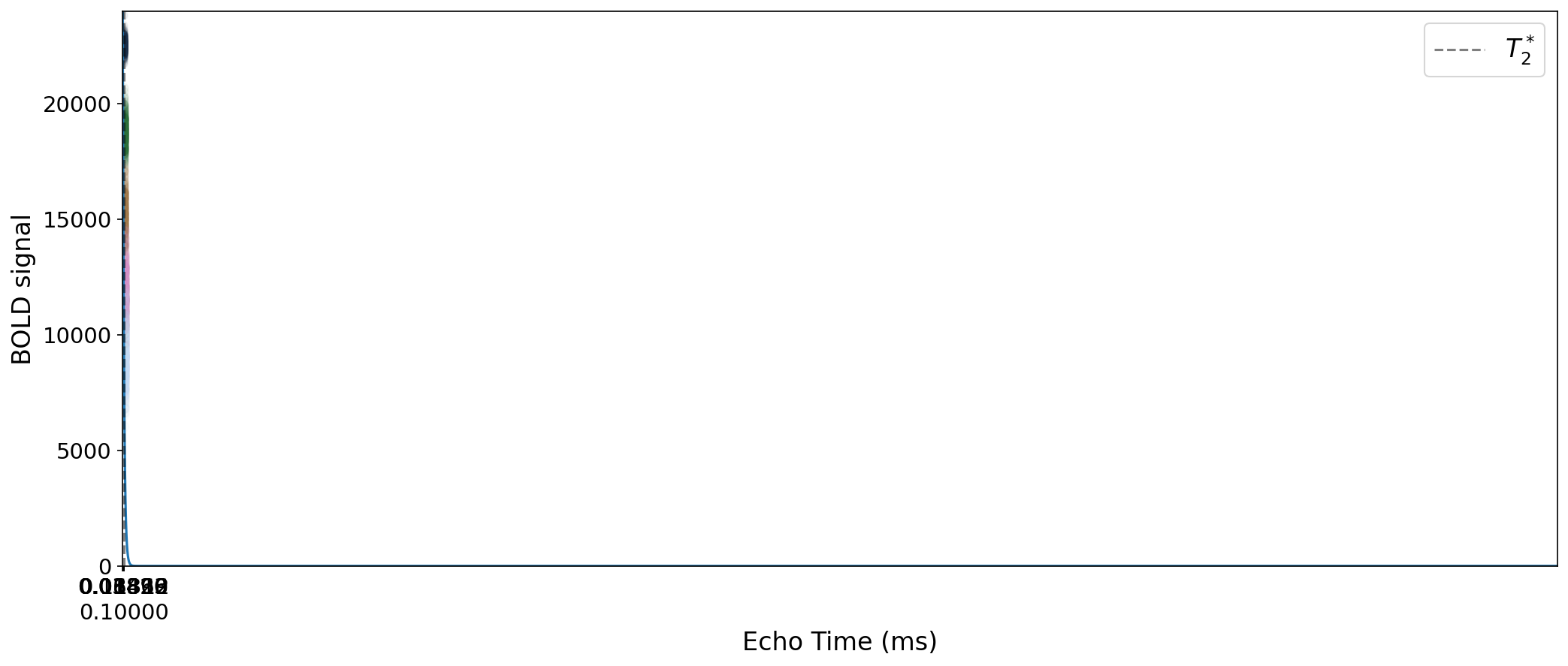
Fig. 28 Scatter plot of voxel’s signal for each echo with T2* estimate.#
Optimal combination weights#
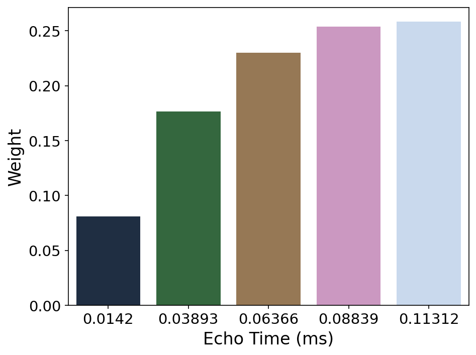
Fig. 29 Averaging weights for optimal combination.#
Optimally combined timeseries#
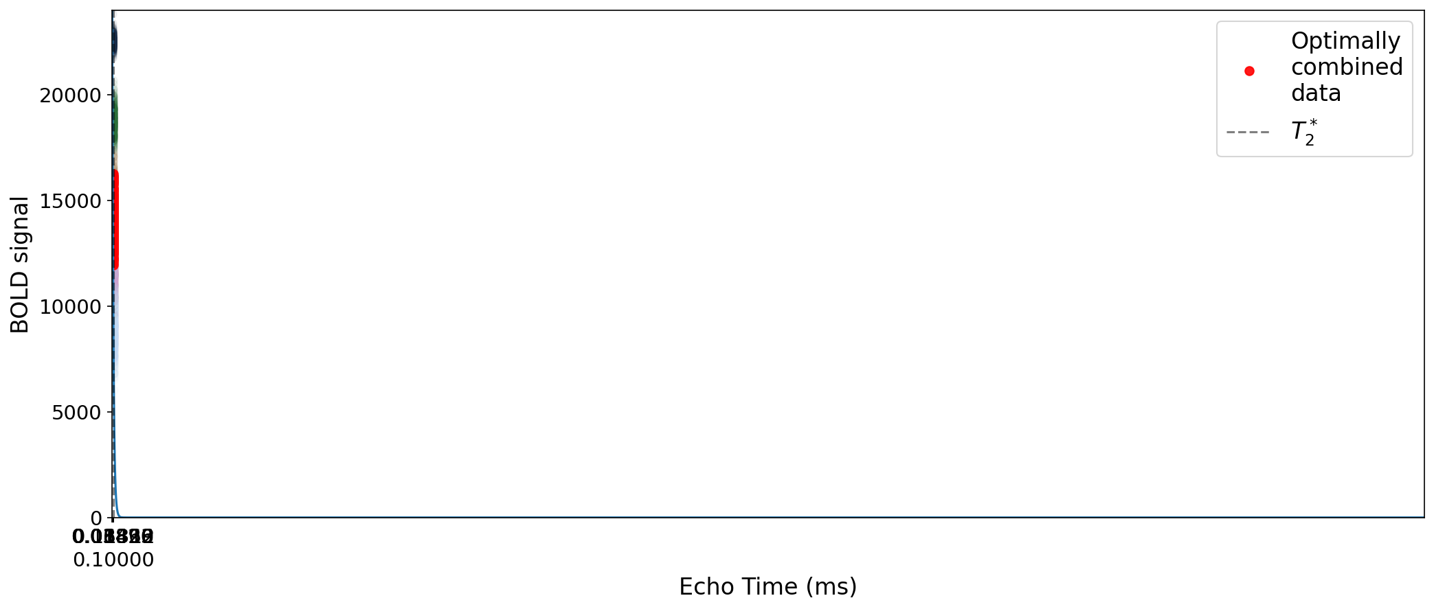
Fig. 30 Scatter plot of voxel’s signal for each echo with optimally combined signal as well.#
Optimally combined timeseries#
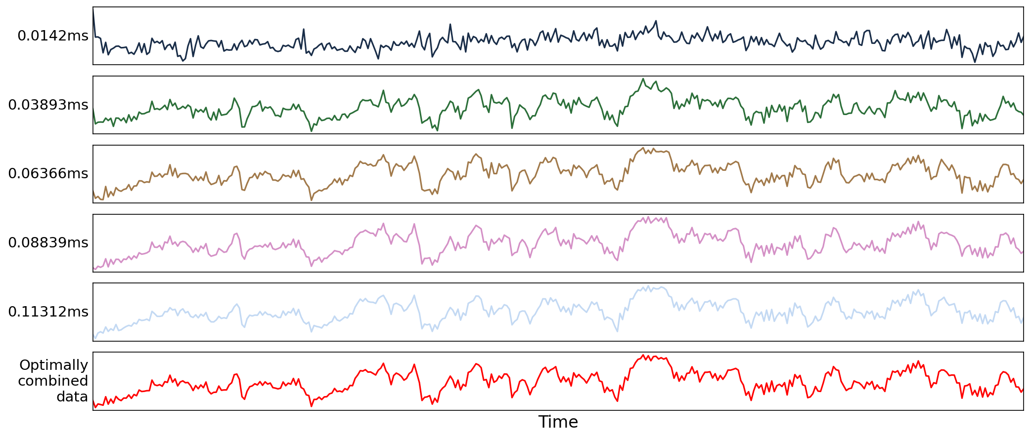
Fig. 31 Echo-wise time series for a voxel, including the optimally combined time series.#
Multi-Echo Principal Components Analysis#
Optimally combined data are decomposed with PCA. The PCA components are selected according to one of multiple possible approaches. Two possible approaches are a decision tree and a threshold using the percentage of variance explained by each component.
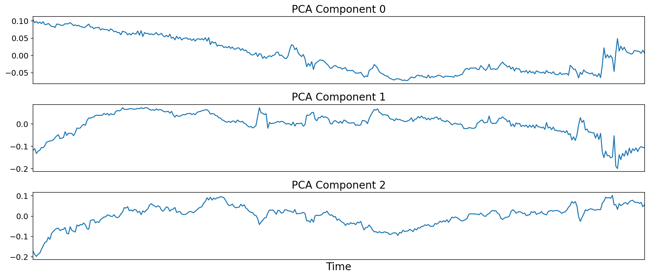
Fig. 32 Time series of three PCA components.#
Data Whitening#
The selected components from the PCA are recombined to produce a whitened version of the optimally combined data.
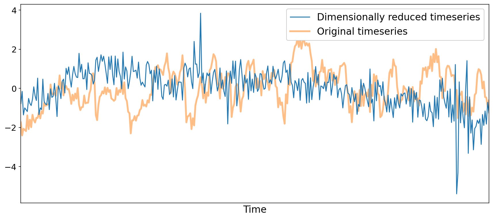
Fig. 33 Time series of optimally combined data from a voxel, before and after dimensionality reduction with PCA.#
Multi-Echo Independent Components Analysis#
The whitened optimally combined data are then decomposed with ICA. The number of ICA components is limited to the number of retained components from the PCA, in order to reflect the true dimensionality of the data. ICA produces a mixing matrix (i.e., timeseries for each component).
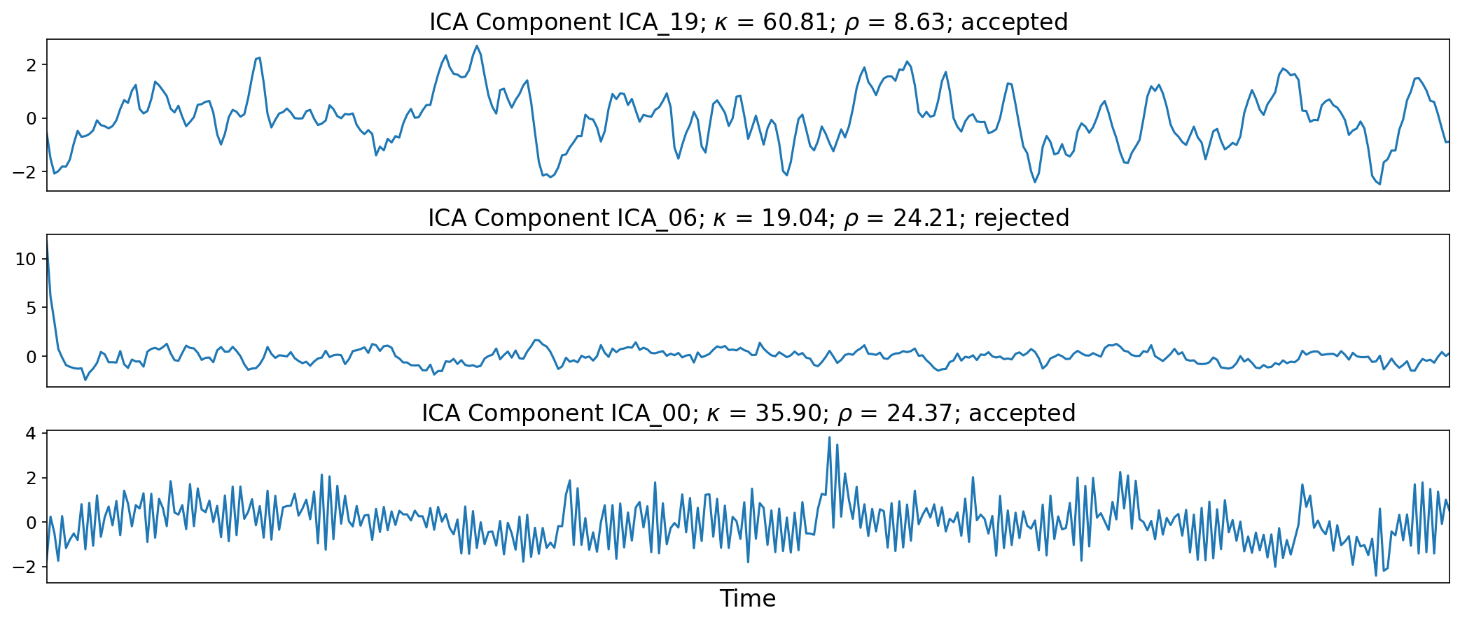
Fig. 34 Time series of three ICA components.#
\(R_2\) and \(S_0\) Model Fit#
Linear regression is used to fit the component timeseries to each voxel in each echo from the original, echo-specific data. This results in echo- and voxel-specific betas for each of the components. TE-dependence (\(R_2\)) and TE-independence (\(S_0\)) models can then be fit to these betas.
These models allow calculation of F-statistics for the \(R_2\) and \(S_0\) models (referred to as \(\kappa\) and \(\rho\), respectively).
Note that the values here are for a single voxel (the highest-weighted one for the component), but \(\kappa\) and \(\rho\) are averaged across voxels.
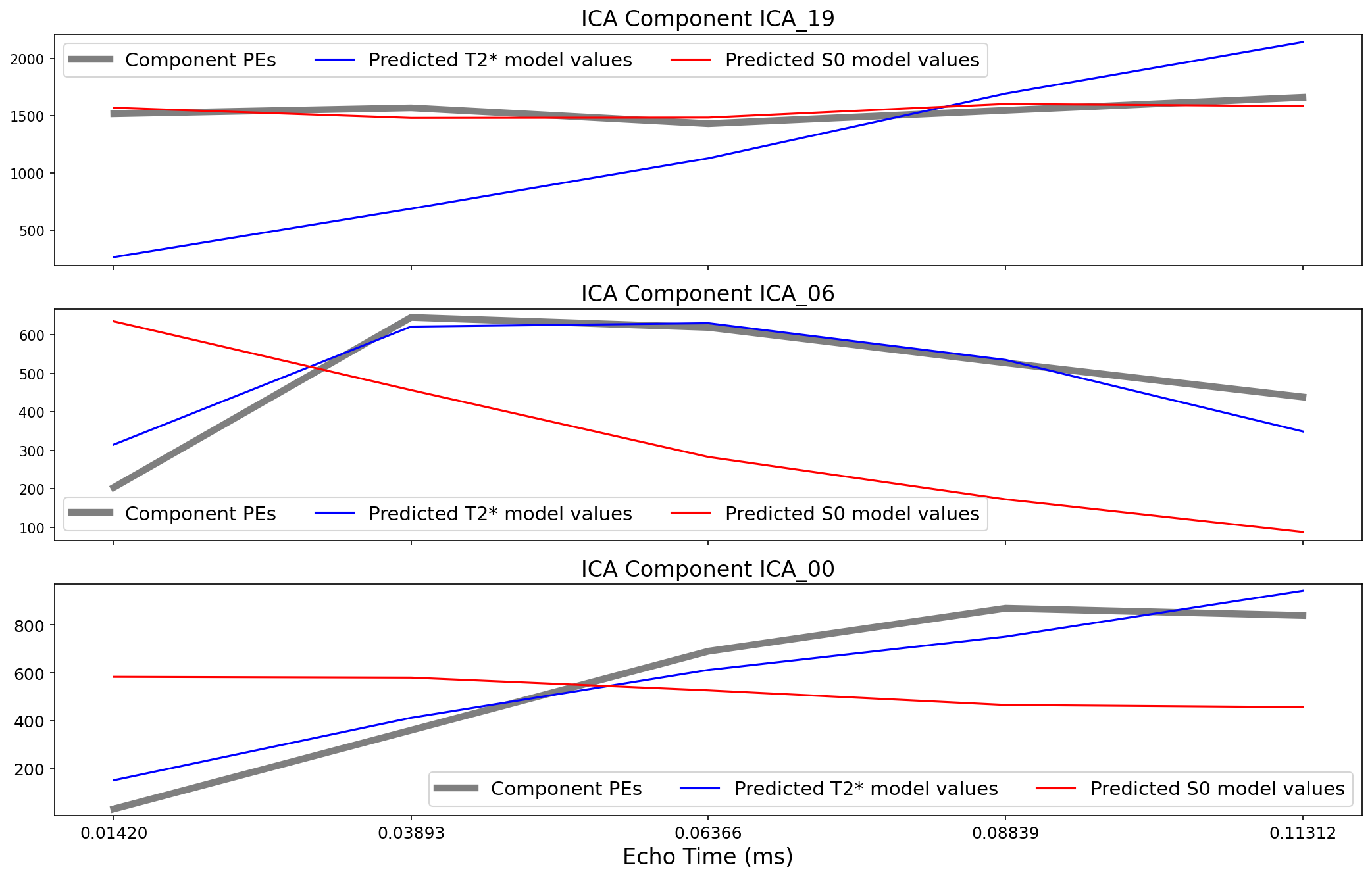
Fig. 35 Echo-wise model weights for three ICA components.#
ICA Component Selection and Multi-Echo Denoising#
A decision tree is applied to \(\kappa\), \(\rho\), and other metrics in order to classify ICA components as TE-dependent (BOLD signal), TE-independent (non-BOLD noise), or neither (to be ignored).
The ICA components are fitted to the original (not whitened) optimally combined data with linear regression, which is used to weight the components for construction of the denoised data. The residuals from this regression will thus include the variance that was not included in the PCA-whitened optimally combined data.
The MEDN dataset is constructed from the accepted (BOLD) and ignored components, as well as the residual variance not explained by the ICA. The MEHK dataset is constructed just from the accepted (BOLD) components. This means that ignored components and residual variance not explained by the ICA are not included in the resulting dataset.
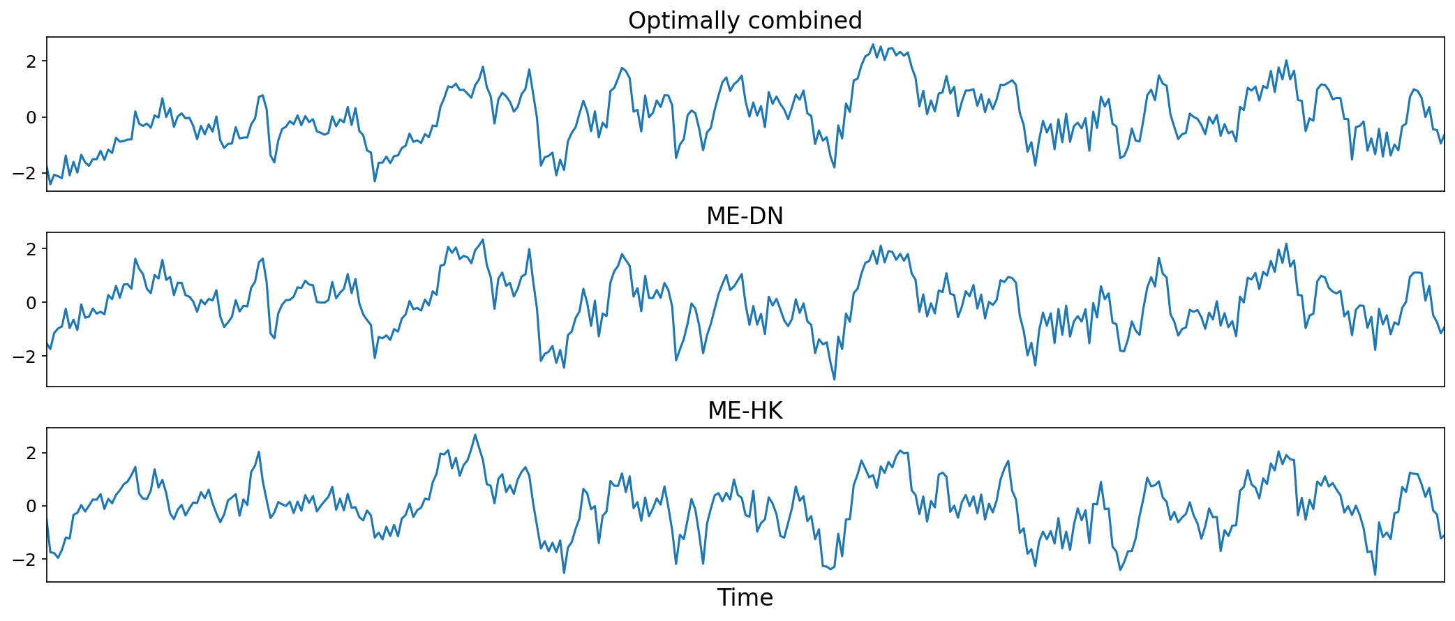
Fig. 36 Time series for optimally combined, denoised, and high-kappa data for a single voxel.#
Post-processing to remove spatially diffuse noise#
Due to the constraints of ICA, MEICA is able to identify and remove spatially localized noise components, but it cannot identify components that are spread out throughout the whole brain.
One of several post-processing strategies may be applied to the ME-DN or ME-HK datasets in order to remove spatially diffuse (ostensibly respiration-related) noise. Methods which have been employed in the past include global signal regression (GSR), Minimum Image Regression, anatomical CompCor, Go Decomposition (GODEC), and robust PCA.
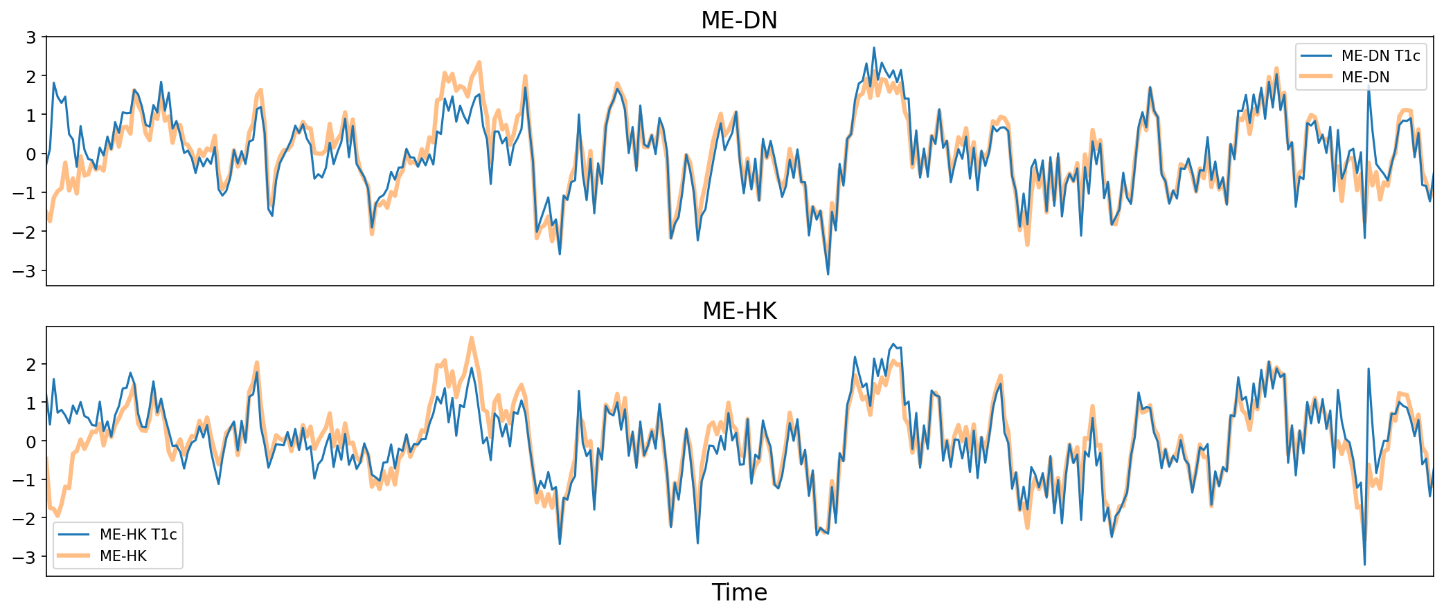
Fig. 37 Time series from a voxel before and after minimum image regression.#