Model-free deconvolution with pySPFM

Multi-echo fMRI lets us estimate neuronal-related activity directly from the BOLD signal without a task model, using Sparse Paradigm Free Mapping (SPFM). pySPFM deconvolves the haemodynamic response from the data and recovers a sparse activity-inducing signal — an estimate of when each region becomes active — like the examples in the pySPFM documentation.

To keep the analysis fast and laptop-friendly we run the deconvolution parcel-wise: averaging voxels within each region of the Schaefer atlas shrinks the problem and boosts SNR, which makes the multi-echo fit well behaved.

Load the multi-echo data

import json
import os
import warnings
from glob import glob

import nibabel as nb
import numpy as np
import matplotlib.pyplot as plt
from nilearn import plotting
from nilearn.datasets import fetch_atlas_schaefer_2018
from nilearn.image import resample_to_img
from nilearn.maskers import NiftiLabelsMasker
from nilearn.signal import clean

warnings.filterwarnings("ignore")

data_path = os.path.abspath("../data")
func_dir = os.path.join(data_path, "ds006185/sub-24053/ses-1/func/")

data_files = sorted(
    glob(
        os.path.join(
            func_dir,
            "sub-24053_ses-1_task-rat_dir-PA_run-01_echo-*_part-mag_desc-preproc_bold.nii.gz",
        ),
    ),
)
mask_file = os.path.join(
    func_dir,
    "sub-24053_ses-1_task-rat_dir-PA_run-01_part-mag_desc-brain_mask.nii.gz",
)

if not data_files:
    raise FileNotFoundError(
        f"No echo files found under {func_dir}. Run the data download in "
        "`00_Download_Data` (datalad get of the task-rat_dir-PA echoes) first."
    )

# Read the echo times (converted to ms) and the repetition time (s) from the BIDS
# JSON sidecars, so the HRF is built with the correct acquisition timing.
echo_times = []
for f in data_files:
    with open(f.replace(".nii.gz", ".json"), "r") as fo:
        metadata = json.load(fo)
    echo_times.append(metadata["EchoTime"] * 1000)
tr = metadata["RepetitionTime"]

out_dir = os.path.join(data_path, "pySPFM")
os.makedirs(out_dir, exist_ok=True)

print(f"{len(data_files)} echoes | TE = {[round(t, 1) for t in echo_times]} ms | TR = {tr} s")

5 echoes | TE = [14.2, 38.9, 63.7, 88.4, 113.1] ms | TR = 1.761 s

Parcellate, detrend and normalise

Each echo is averaged within Schaefer parcels (restricted to the brain mask), then detrended and band-pass filtered (0.01–0.1 Hz), and only then converted to percent signal change. The order matters: we strip drift and out-of-band fluctuations first, then express what remains as a fraction of the parcel’s baseline.

• Detrending and band-pass filtering — scanner drift (below 0.01 Hz) and high-frequency noise (above 0.1 Hz, e.g. residual cardiac/respiratory and thermal noise) are not part of the haemodynamic response, so we keep only the 0.01–0.1 Hz band where the BOLD response lives.

• Normalisation to percent signal change — pySPFM expects normalised input; feeding raw signal intensities collapses the deconvolution to zero.

# Schaefer cortical parcellation. Averaging within ~400 parcels reduces the problem
# from ~218k voxels to a few hundred ROIs and improves SNR. Increase n_rois for a
# finer map at the cost of a longer fit.
# Download the atlas into the git-ignored ../data tree instead of the default
# ~/nilearn_data, so it does not clutter the user's home directory.
atlas = fetch_atlas_schaefer_2018(n_rois=400, data_dir=os.path.join(data_path, "nilearn"))

masker = NiftiLabelsMasker(
    labels_img=atlas.maps,
    mask_img=mask_file,        # only average voxels inside the brain
    resampling_target="data",  # resample the atlas onto the fMRI's native grid
    standardize=False,
)
masker.fit(data_files[0])

masked_data = []
for f in data_files:
    echo_data = masker.transform(f)  # (n_timepoints, n_parcels)
    # Detrend and band-pass (0.01-0.1 Hz) first, then normalise: express the cleaned
    # signal as a fraction of the parcel's raw baseline mean (percent signal change).
    baseline = echo_data.mean(axis=0, keepdims=True)
    detrended = clean(
        echo_data, detrend=True, low_pass=0.1, high_pass=0.01, t_r=tr, standardize=False
    )
    with np.errstate(invalid="ignore", divide="ignore"):
        pc = detrended / baseline  # percent signal change
    masked_data.append(pc)

X = np.vstack(masked_data)  # (n_echoes * n_timepoints, n_parcels)
n_scans = X.shape[0] // len(data_files)

# Drop parcels that fall outside the field of view (empty/constant after masking).
valid = np.all(np.isfinite(X), axis=0) & (X.std(axis=0) > 0)
X = X[:, valid]

print(f"Input matrix: {X.shape}  ({len(data_files)} echoes x {n_scans} TRs, {X.shape[1]} parcels)")

[fetch_atlas_schaefer_2018] Dataset found in /Users/eurunuela/GitHub/multi-echo-data-analysis/data/nilearn/schaefer_2018

Input matrix: (1815, 358)  (5 echoes x 363 TRs, 358 parcels)

Deconvolve: the effect of the model-selection criterion

pySPFM selects the amount of regularisation (i.e. how sparse the estimate is) automatically from a criterion. We compare the two LARS-based criteria for the multi-echo model:

• bic — a strong complexity penalty, so it keeps only the few most confident events (a very sparse estimate).

• aic — a lighter penalty, so it recovers activity-inducing events across most of the brain.

(The FISTA-based criteria such as mad are not numerically stable for the multi-echo model on these data, so we stick to the LARS criteria.)

from pySPFM import SparseDeconvolution

models = {}
for criterion in ["bic", "aic"]:
    model = SparseDeconvolution(tr=tr, te=echo_times, criterion=criterion)
    model.fit(X)
    models[criterion] = model
    active = np.mean(np.any(model.coef_ != 0, axis=0)) * 100
    print(f"{criterion.upper()}: {active:.0f}% of parcels show activity")

# Guard against a silently degenerate fit (e.g. wrong scaling or TR).
assert np.any(models["aic"].coef_ != 0), "Deconvolution returned all zeros — check normalisation/TR."

np.save(os.path.join(out_dir, "out_activity_bic.npy"), models["bic"].coef_)
np.save(os.path.join(out_dir, "out_activity_aic.npy"), models["aic"].coef_)

dask configuration wasn't detected, if you are using a cluster please look at the jobqueue YAML example, modify it so it works in your cluster and add it to ~/.config/dask local configuration will be used.You can find a jobqueue YAML example in the pySPFM/jobqueue.yaml file.

BIC: 65% of parcels show activity

dask configuration wasn't detected, if you are using a cluster please look at the jobqueue YAML example, modify it so it works in your cluster and add it to ~/.config/dask local configuration will be used.You can find a jobqueue YAML example in the pySPFM/jobqueue.yaml file.

AIC: 96% of parcels show activity

A single parcel: BIC vs. AIC

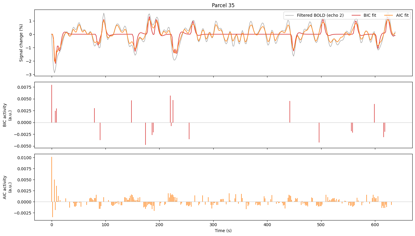
For one representative parcel: the band-pass-filtered BOLD (echo 2) with each model’s fit, and the activity-inducing signal recovered by each criterion. BIC keeps only a handful of strong events; AIC recovers many more — the same trade-off illustrated in the pySPFM documentation.

echo2 = masked_data[1][:, valid]                                   # filtered echo-2 % change
coef_bic, coef_aic = models["bic"].coef_, models["aic"].coef_
fit_bic = models["bic"].get_fitted_signal()[n_scans:2 * n_scans, :]
fit_aic = models["aic"].get_fitted_signal()[n_scans:2 * n_scans, :]

# Representative parcel: active in BIC, realistic amplitude, best AIC fit to the data.
amplitude = echo2.std(axis=0)
candidates = np.where(np.any(coef_bic != 0, axis=0) & (amplitude > 0.003) & (amplitude < 0.04))[0]
if candidates.size == 0:  # fall back to any active parcel
    candidates = np.where(np.any(coef_aic != 0, axis=0))[0]
corr = np.array([np.corrcoef(fit_aic[:, i], echo2[:, i])[0, 1] for i in candidates])
parcel = int(candidates[int(np.argmax(corr))])

t = np.arange(n_scans) * tr
fig, axes = plt.subplots(3, 1, figsize=(14, 8), sharex=True)
axes[0].plot(t, echo2[:, parcel] * 100, color="0.6", lw=1.0, label="Filtered BOLD (echo 2)")
axes[0].plot(t, fit_bic[:, parcel] * 100, color="tab:red", lw=1.3, label="BIC fit")
axes[0].plot(t, fit_aic[:, parcel] * 100, color="tab:orange", lw=1.3, label="AIC fit")
axes[0].set_ylabel("Signal change (%)")
axes[0].set_title(f"Parcel {parcel}")
axes[0].legend(loc="upper right", ncol=3)
axes[1].vlines(t, 0, coef_bic[:, parcel], color="tab:red", lw=1.2)
axes[1].axhline(0, color="0.7", lw=0.6)
axes[1].set_ylabel("BIC activity\n(a.u.)")
axes[2].vlines(t, 0, coef_aic[:, parcel], color="tab:orange", lw=1.2)
axes[2].axhline(0, color="0.7", lw=0.6)
axes[2].set_ylabel("AIC activity\n(a.u.)")
axes[2].set_xlabel("Time (s)")
fig.tight_layout()

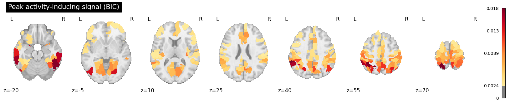
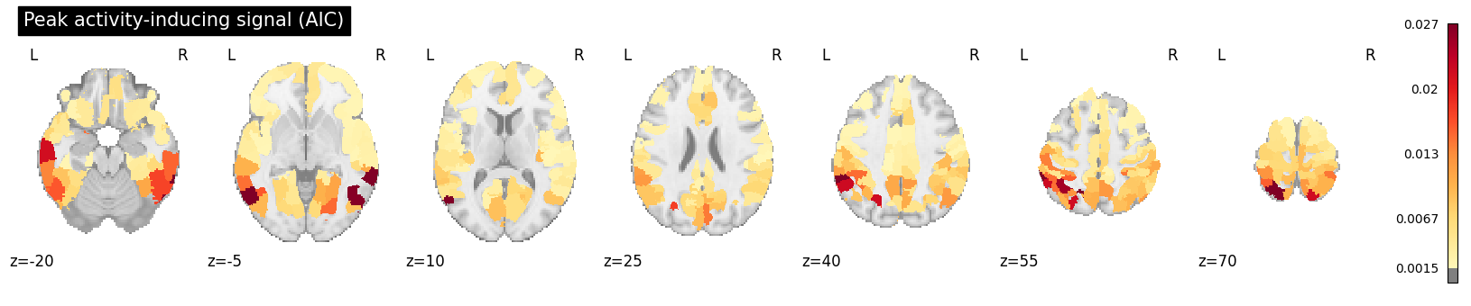
Whole-brain activity: BIC vs. AIC

The peak activity-inducing magnitude of each parcel, shown in MNI space. The multi-echo data are in the subject’s native space and are only affinely aligned to MNI, so we map each parcel’s value onto the original (MNI) Schaefer atlas: inverse_transform would instead land on the native grid and would not line up with the MNI template. Because the parcels were sampled in native space, the anatomical labelling is approximate — good enough for a qualitative whole-brain map, not for precise localisation. BIC highlights only a few strong regions, while AIC reveals activity across most of the cortex.

# The Schaefer atlas is defined in MNI space; the masker orders parcels by ascending
# label id and keeps those with voxels inside the brain mask. Recover that label
# order so each parcel's value can be painted back onto the MNI atlas.
atlas_img = nb.load(atlas.maps)
atlas_data = np.asarray(atlas_img.dataobj).astype(int)
atlas_on_data = resample_to_img(
    atlas_img, nb.load(mask_file), interpolation="nearest", force_resample=True, copy_header=True
).get_fdata().astype(int)
brain = nb.load(mask_file).get_fdata() > 0
labels = np.array(sorted(np.unique(atlas_on_data[brain & (atlas_on_data > 0)])))
assert labels.size == models["aic"].coef_.shape[1], "parcel/label count mismatch"

def peak_activity_map(coef):
    peak = np.abs(coef).max(axis=0)  # one value per parcel
    painted = np.zeros(atlas_data.shape)
    for value, label in zip(peak, labels):
        painted[atlas_data == label] = value
    return nb.Nifti1Image(painted, atlas_img.affine), peak

for criterion in ["bic", "aic"]:
    activity_img, peak = peak_activity_map(models[criterion].coef_)
    nonzero = peak[peak > 0]
    plotting.plot_stat_map(
        activity_img,
        display_mode="z",
        cut_coords=[-20, -5, 10, 25, 40, 55, 70],
        threshold=float(np.percentile(nonzero, 10)),
        vmax=float(np.percentile(nonzero, 99)),
        cmap="YlOrRd",
        symmetric_cbar=False,
        title=f"Peak activity-inducing signal ({criterion.upper()})",
        draw_cross=False,
    )

# Save the AIC whole-brain map (MNI space) for reference.
peak_activity_map(models["aic"].coef_)[0].to_filename(
    os.path.join(out_dir, "out_activity_max_aic.nii.gz")
)