Volume-wise T2*/S0 estimation with t2smap

Use tedana.workflows.t2smap_workflow() [DuPre et al., 2021] to calculate volume-wise T2*/S0, as in Power et al. [2018] and Heunis et al. [2021].

import json
import os
from glob import glob

import matplotlib.pyplot as plt
import nibabel as nb
import numpy as np
from IPython import display
from book_utils import glue_figure, load_pafin
from nilearn import image, masking, plotting
from tedana import workflows

data_path = os.path.abspath('../data')

/home/tsalo/micromamba/envs/meda/lib/python3.12/site-packages/requests/__init__.py:113: RequestsDependencyWarning: urllib3 (2.6.3) or chardet (7.2.0)/charset_normalizer (3.4.6) doesn't match a supported version!
  warnings.warn(

/home/tsalo/micromamba/envs/meda/lib/python3.12/site-packages/tqdm/auto.py:21: TqdmWarning: IProgress not found. Please update jupyter and ipywidgets. See https://ipywidgets.readthedocs.io/en/stable/user_install.html
  from .autonotebook import tqdm as notebook_tqdm

data = load_pafin(data_path)
out_dir = os.path.join(data_path, "fit")

workflows.t2smap_workflow(
    data['echo_files'],
    data['echo_times'],
    out_dir=out_dir,
    mask=data['mask'],
    prefix="sub-24053_ses-1_task-rat_dir-PA_run-01_",
    fittype="loglin",
    fitmode="ts",
    overwrite=True,
)

Show code cell output

Hide code cell output

INFO     t2smap:t2smap_workflow:365 Using output directory: /mnt/c/Users/tsalo/Documents/ME-ICA/multi-echo-data-analysis/data/fit

INFO     utils:check_te_values:792 TE values appear to be in seconds. Converting to milliseconds for internal use.

INFO     utils:load_mask:916 Using user-defined mask

INFO     t2smap:t2smap_workflow:426 Loading input data: ['/mnt/c/Users/tsalo/Documents/ME-ICA/multi-echo-data-analysis/data/ds006185/sub-24053/ses-1/func/sub-24053_ses-1_task-rat_dir-PA_run-01_echo-1_part-mag_desc-preproc_bold.nii.gz', '/mnt/c/Users/tsalo/Documents/ME-ICA/multi-echo-data-analysis/data/ds006185/sub-24053/ses-1/func/sub-24053_ses-1_task-rat_dir-PA_run-01_echo-2_part-mag_desc-preproc_bold.nii.gz', '/mnt/c/Users/tsalo/Documents/ME-ICA/multi-echo-data-analysis/data/ds006185/sub-24053/ses-1/func/sub-24053_ses-1_task-rat_dir-PA_run-01_echo-3_part-mag_desc-preproc_bold.nii.gz', '/mnt/c/Users/tsalo/Documents/ME-ICA/multi-echo-data-analysis/data/ds006185/sub-24053/ses-1/func/sub-24053_ses-1_task-rat_dir-PA_run-01_echo-4_part-mag_desc-preproc_bold.nii.gz', '/mnt/c/Users/tsalo/Documents/ME-ICA/multi-echo-data-analysis/data/ds006185/sub-24053/ses-1/func/sub-24053_ses-1_task-rat_dir-PA_run-01_echo-5_part-mag_desc-preproc_bold.nii.gz']

INFO     utils:make_adaptive_mask:167 Echo-wise intensity thresholds for adaptive mask: [5390.2476 3376.5105 1811.7682 1076.2314  610.8774]

WARNING  utils:make_adaptive_mask:195 9757 voxels in user-defined mask do not have good signal. Removing voxels from mask.

INFO     t2smap:t2smap_workflow:456 Computing T2* map

INFO     t2smap:t2smap_workflow:503 Calculating model fit quality metrics

INFO     t2smap:t2smap_workflow:519 Computing optimal combination

INFO     combine:make_optcom:202 Optimally combining data with voxel- and volume-wise T2* estimates

INFO     t2smap:t2smap_workflow:564 Workflow completed

INFO     utils:log_newsletter_info:812 Don't forget to subscribe to the tedana newsletter for updates! This is a very low volume email list.

INFO     utils:log_newsletter_info:816 https://groups.google.com/g/tedana-newsletter

out_files = sorted(glob(os.path.join(out_dir, "*")))
out_files = [os.path.basename(f) for f in out_files]
print("\n".join(out_files))

figures
sub-24053_ses-1_task-rat_dir-PA_run-01_S0map.nii.gz
sub-24053_ses-1_task-rat_dir-PA_run-01_T2starmap.nii.gz
sub-24053_ses-1_task-rat_dir-PA_run-01_dataset_description.json
sub-24053_ses-1_task-rat_dir-PA_run-01_desc-adaptiveGoodSignal_mask.nii.gz
sub-24053_ses-1_task-rat_dir-PA_run-01_desc-confounds_timeseries.tsv
sub-24053_ses-1_task-rat_dir-PA_run-01_desc-limited_S0map.nii.gz
sub-24053_ses-1_task-rat_dir-PA_run-01_desc-limited_T2starmap.nii.gz
sub-24053_ses-1_task-rat_dir-PA_run-01_desc-optcom_bold.nii.gz
sub-24053_ses-1_task-rat_dir-PA_run-01_desc-rmse_statmap.nii.gz
sub-24053_ses-1_task-rat_dir-PA_run-01_desc-tedana_registry.json

fig, axes = plt.subplots(figsize=(16, 16), nrows=3)

plotting.plot_carpet(
    os.path.join(out_dir, "sub-24053_ses-1_task-rat_dir-PA_run-01_desc-optcom_bold.nii.gz"),
    axes=axes[0],
    figure=fig,
)
axes[0].set_title("Optimally Combined Data", fontsize=20)
plotting.plot_carpet(
    os.path.join(out_dir, "sub-24053_ses-1_task-rat_dir-PA_run-01_T2starmap.nii.gz"),
    axes=axes[1],
    figure=fig,
)
axes[1].set_title("T2* Estimates", fontsize=20)
plotting.plot_carpet(
    os.path.join(out_dir, "sub-24053_ses-1_task-rat_dir-PA_run-01_S0map.nii.gz"),
    axes=axes[2],
    figure=fig,
)
axes[2].set_title("S0 Estimates", fontsize=20)
axes[0].xaxis.set_visible(False)
axes[1].xaxis.set_visible(False)
axes[0].spines["bottom"].set_visible(False)
axes[1].spines["bottom"].set_visible(False)
fig.tight_layout()

glue_figure("figure_volumewise_t2ss0_carpets", fig, display=False)

Show code cell output

Hide code cell output

/tmp/ipykernel_6771/2185078944.py:3: DeprecationWarning: The default strategy for standardize is currently 'zscore' which incorrectly uses population std to calculate sample zscores. The new strategy 'zscore_sample' corrects this behavior by using the sample std. In release 0.13, the default strategy will be replaced by the new strategy and the 'zscore' option will be removed. Please use 'zscore_sample' instead.
  plotting.plot_carpet(

/tmp/ipykernel_6771/2185078944.py:9: DeprecationWarning: The default strategy for standardize is currently 'zscore' which incorrectly uses population std to calculate sample zscores. The new strategy 'zscore_sample' corrects this behavior by using the sample std. In release 0.13, the default strategy will be replaced by the new strategy and the 'zscore' option will be removed. Please use 'zscore_sample' instead.
  plotting.plot_carpet(

/tmp/ipykernel_6771/2185078944.py:15: DeprecationWarning: The default strategy for standardize is currently 'zscore' which incorrectly uses population std to calculate sample zscores. The new strategy 'zscore_sample' corrects this behavior by using the sample std. In release 0.13, the default strategy will be replaced by the new strategy and the 'zscore' option will be removed. Please use 'zscore_sample' instead.
  plotting.plot_carpet(

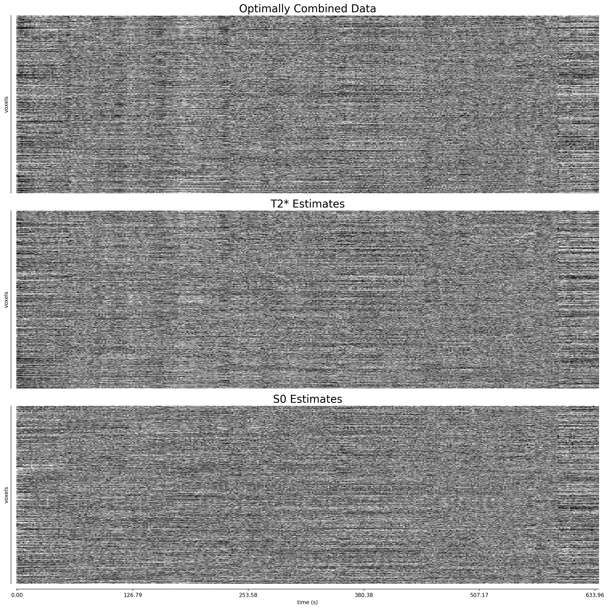
Fig. 28 Carpet plots of optimally combined data, along with volume-wise T2* and S0 estimates.

fig, ax = plt.subplots(figsize=(16, 8))
in_file = image.mean_img(
    os.path.join(out_dir, "sub-24053_ses-1_task-rat_dir-PA_run-01_T2starmap.nii.gz")
)
arr = masking.apply_mask(in_file, data['mask'])
thresh = np.nanpercentile(arr, 98)
plotting.plot_stat_map(
    in_file,
    draw_cross=False,
    bg_img=None,
    figure=fig,
    axes=ax,
    cmap="Reds",
    vmin=0,
    vmax=thresh,
)
glue_figure("figure_mean_volumewise_t2s", fig, display=False)

Show code cell output

Hide code cell output

/tmp/ipykernel_6771/3336080904.py:2: FutureWarning: From release 0.13.0 onwards, this function will, by default, copy the header of the input image to the output. Currently, the header is reset to the default Nifti1Header. To suppress this warning and use the new behavior, set `copy_header=True`.
  in_file = image.mean_img(

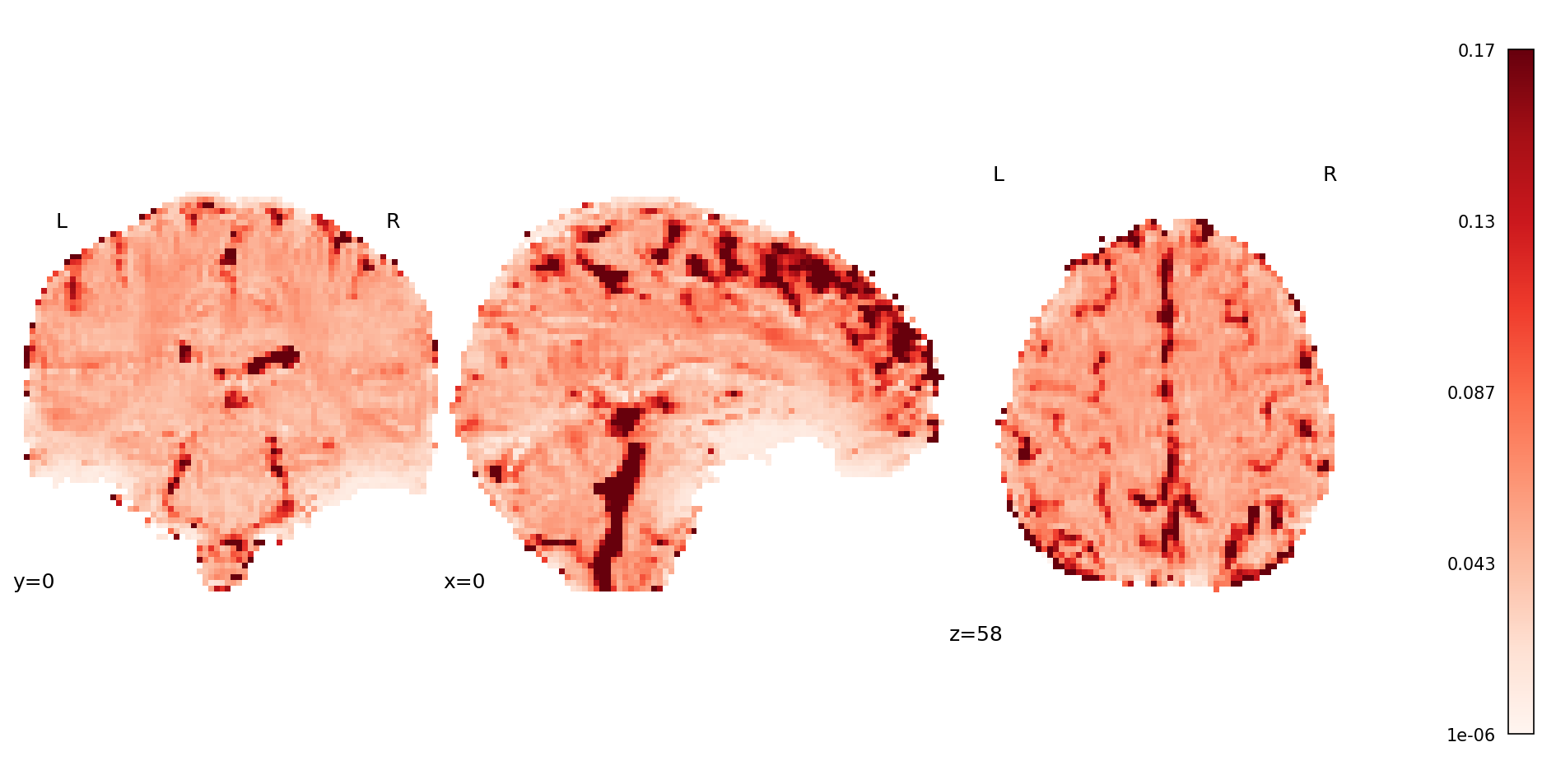
Fig. 29 Mean map from the volume-wise T2* estimation.

fig, ax = plt.subplots(figsize=(16, 8))
in_file = image.mean_img(
    os.path.join(out_dir, "sub-24053_ses-1_task-rat_dir-PA_run-01_S0map.nii.gz")
)
arr = masking.apply_mask(in_file, data['mask'])
thresh = np.nanpercentile(arr, 98)
plotting.plot_stat_map(
    in_file,
    draw_cross=False,
    bg_img=None,
    figure=fig,
    axes=ax,
    cmap="Reds",
    vmin=0,
    vmax=thresh,
)
glue_figure("figure_mean_volumewise_s0", fig, display=False)

Show code cell output

Hide code cell output

/tmp/ipykernel_6771/1178446598.py:2: FutureWarning: From release 0.13.0 onwards, this function will, by default, copy the header of the input image to the output. Currently, the header is reset to the default Nifti1Header. To suppress this warning and use the new behavior, set `copy_header=True`.
  in_file = image.mean_img(

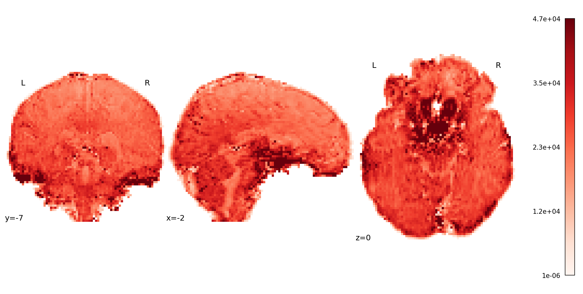
Fig. 30 Mean map from the volume-wise S0 estimation.

fig, axes = plt.subplots(figsize=(16, 15), nrows=5)
plotting.plot_epi(
    image.mean_img(data['echo_files'][0]),
    draw_cross=False,
    bg_img=None,
    cut_coords=[-10, 0, 10, 20, 30, 40, 50, 60, 70],
    display_mode="z",
    axes=axes[0],
)
plotting.plot_epi(
    image.mean_img(data['echo_files'][1]),
    draw_cross=False,
    bg_img=None,
    cut_coords=[-10, 0, 10, 20, 30, 40, 50, 60, 70],
    display_mode="z",
    axes=axes[1],
)
plotting.plot_epi(
    image.mean_img(data['echo_files'][2]),
    draw_cross=False,
    bg_img=None,
    cut_coords=[-10, 0, 10, 20, 30, 40, 50, 60, 70],
    display_mode="z",
    axes=axes[2],
)
plotting.plot_epi(
    image.mean_img(data['echo_files'][3]),
    draw_cross=False,
    bg_img=None,
    cut_coords=[-10, 0, 10, 20, 30, 40, 50, 60, 70],
    display_mode="z",
    axes=axes[3],
)
plotting.plot_epi(
    image.mean_img(
        os.path.join(
            out_dir, "sub-24053_ses-1_task-rat_dir-PA_run-01_desc-optcom_bold.nii.gz"
        )
    ),
    draw_cross=False,
    bg_img=None,
    cut_coords=[-10, 0, 10, 20, 30, 40, 50, 60, 70],
    display_mode="z",
    axes=axes[4],
)
glue_figure("figure_mean_echos_and_optcom", fig, display=False)

Show code cell output

Hide code cell output

/tmp/ipykernel_6771/1298998139.py:3: FutureWarning: From release 0.13.0 onwards, this function will, by default, copy the header of the input image to the output. Currently, the header is reset to the default Nifti1Header. To suppress this warning and use the new behavior, set `copy_header=True`.
  image.mean_img(data['echo_files'][0]),

/tmp/ipykernel_6771/1298998139.py:11: FutureWarning: From release 0.13.0 onwards, this function will, by default, copy the header of the input image to the output. Currently, the header is reset to the default Nifti1Header. To suppress this warning and use the new behavior, set `copy_header=True`.
  image.mean_img(data['echo_files'][1]),

/tmp/ipykernel_6771/1298998139.py:19: FutureWarning: From release 0.13.0 onwards, this function will, by default, copy the header of the input image to the output. Currently, the header is reset to the default Nifti1Header. To suppress this warning and use the new behavior, set `copy_header=True`.
  image.mean_img(data['echo_files'][2]),

/tmp/ipykernel_6771/1298998139.py:27: FutureWarning: From release 0.13.0 onwards, this function will, by default, copy the header of the input image to the output. Currently, the header is reset to the default Nifti1Header. To suppress this warning and use the new behavior, set `copy_header=True`.
  image.mean_img(data['echo_files'][3]),

/tmp/ipykernel_6771/1298998139.py:35: FutureWarning: From release 0.13.0 onwards, this function will, by default, copy the header of the input image to the output. Currently, the header is reset to the default Nifti1Header. To suppress this warning and use the new behavior, set `copy_header=True`.
  image.mean_img(

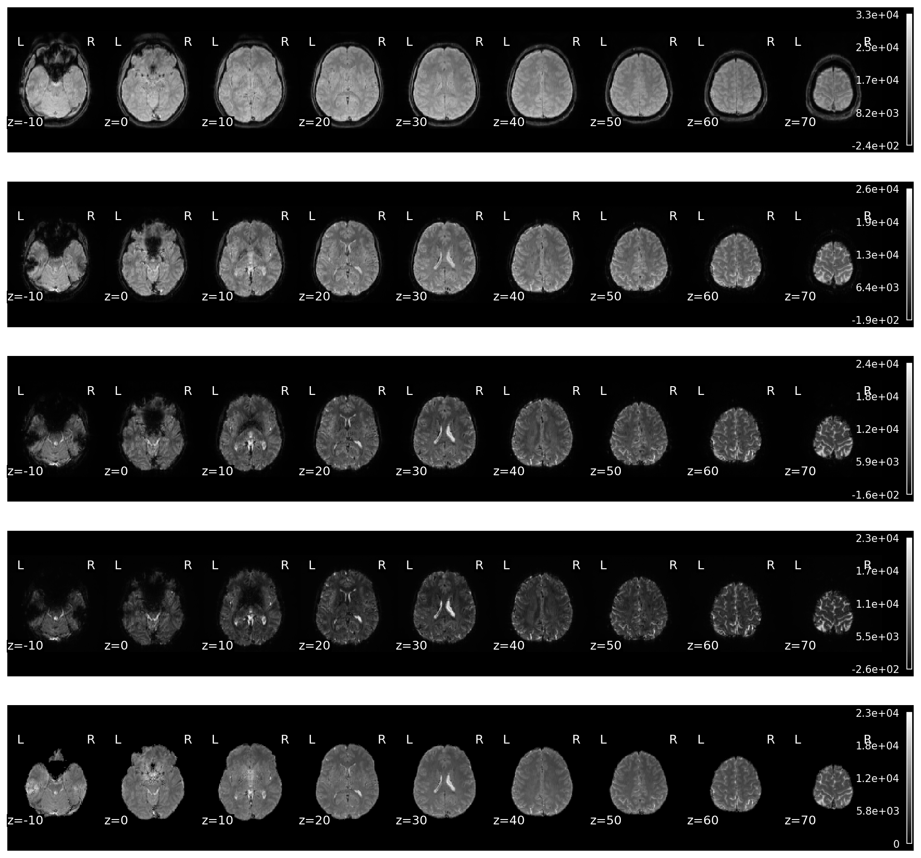
Fig. 31 Mean images of the echo-wise data and the optimally combined data.

te30_tsnr = image.math_img(
    "(np.nanmean(img, axis=3) / np.nanstd(img, axis=3)) * mask",
    img=data['echo_files'][1],
    mask=data['mask'],
)
oc_tsnr = image.math_img(
    "(np.nanmean(img, axis=3) / np.nanstd(img, axis=3)) * mask",
    img=os.path.join(
        out_dir, "sub-24053_ses-1_task-rat_dir-PA_run-01_desc-optcom_bold.nii.gz"
    ),
    mask=data['mask'],
)
arr = masking.apply_mask(te30_tsnr, data['mask'])
thresh = np.nanpercentile(arr, 98)
arr = masking.apply_mask(oc_tsnr, data['mask'])
thresh = np.maximum(thresh, np.nanpercentile(arr, 98))

fig, axes = plt.subplots(figsize=(10, 8), nrows=2)
plotting.plot_stat_map(
    te30_tsnr,
    draw_cross=False,
    bg_img=None,
    threshold=0.1,
    cut_coords=[0, 10, 10],
    symmetric_cbar=False,
    axes=axes[0],
    cmap="Reds",
    vmin=0,
    vmax=thresh,
)
axes[0].set_title("TE30 TSNR", fontsize=16)
plotting.plot_stat_map(
    oc_tsnr,
    draw_cross=False,
    bg_img=None,
    threshold=0.1,
    cut_coords=[0, 10, 10],
    symmetric_cbar=False,
    axes=axes[1],
    cmap="Reds",
    vmin=0,
    vmax=thresh,
)
axes[1].set_title("Optimal Combination TSNR", fontsize=16)
glue_figure("figure_t2snr_te30_and_optcom", fig, display=False)

Show code cell output

Hide code cell output

<string>:1: RuntimeWarning: invalid value encountered in divide

/tmp/ipykernel_6771/3685653445.py:32: UserWarning: Non-finite values detected. These values will be replaced with zeros.
  plotting.plot_stat_map(

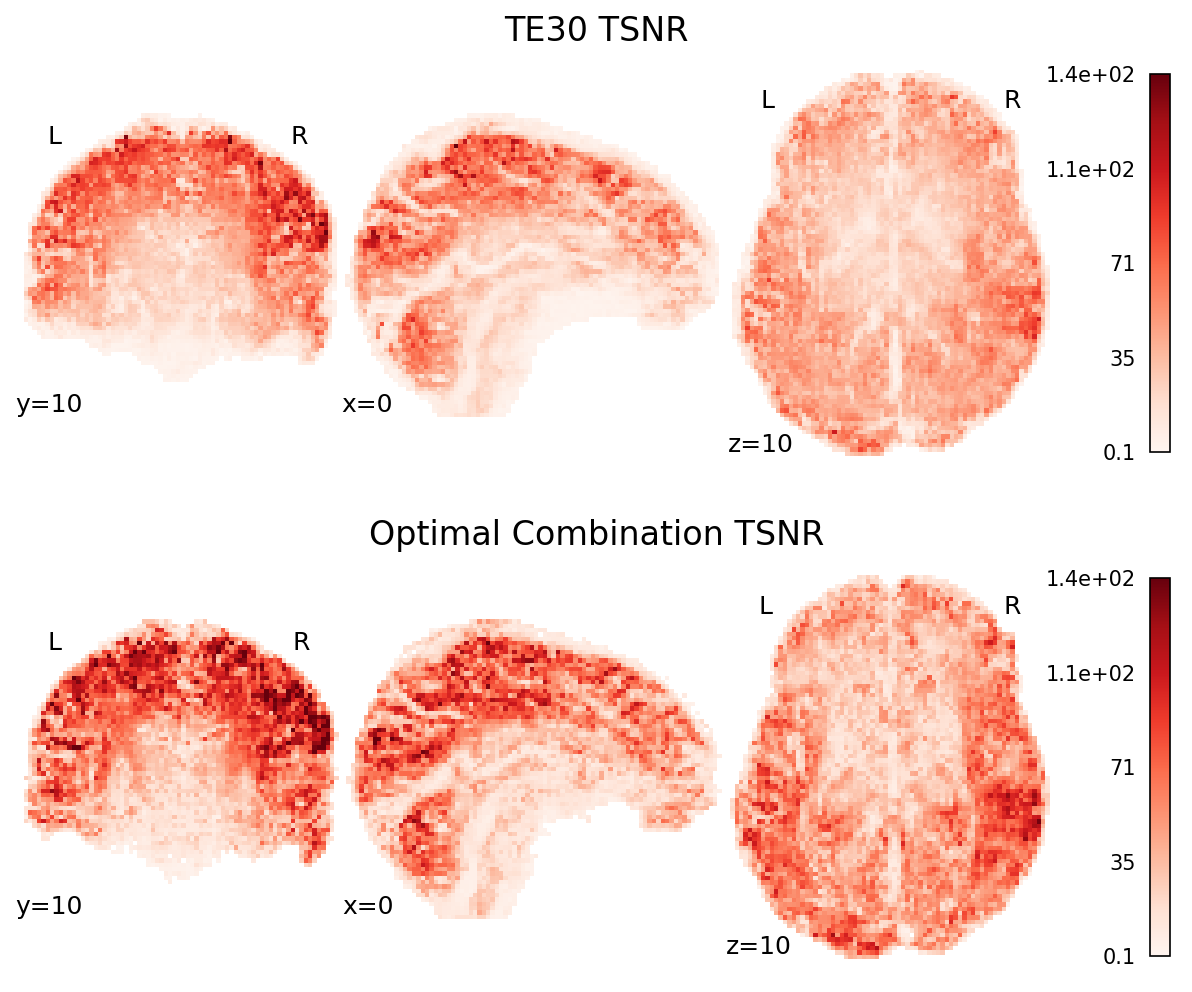
Fig. 32 TSNR map of the second echo (TE30) and the optimally combined data.

fig, ax = plt.subplots(figsize=(16, 8))
plotting.plot_carpet(
    data['echo_files'][1],
    axes=ax,
)
glue_figure("figure_echo3_carpet", fig, display=False)

Show code cell output

Hide code cell output

/tmp/ipykernel_6771/582452611.py:2: DeprecationWarning: The default strategy for standardize is currently 'zscore' which incorrectly uses population std to calculate sample zscores. The new strategy 'zscore_sample' corrects this behavior by using the sample std. In release 0.13, the default strategy will be replaced by the new strategy and the 'zscore' option will be removed. Please use 'zscore_sample' instead.
  plotting.plot_carpet(

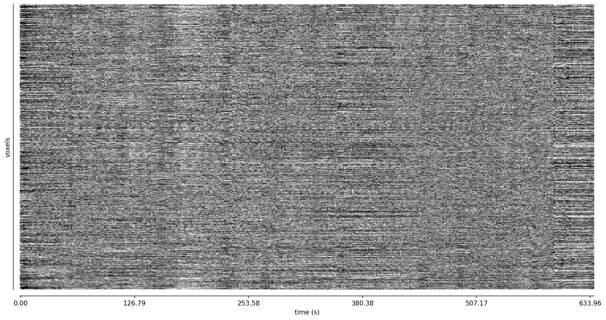
Fig. 33 Carpet plot of the third echo.

fig, ax = plt.subplots(figsize=(16, 8))
plotting.plot_carpet(
    os.path.join(out_dir, "sub-24053_ses-1_task-rat_dir-PA_run-01_desc-optcom_bold.nii.gz"),
    axes=ax,
)
glue_figure("figure_carpet_optcom", fig, display=False)

Show code cell output

Hide code cell output

/tmp/ipykernel_6771/3924763795.py:2: DeprecationWarning: The default strategy for standardize is currently 'zscore' which incorrectly uses population std to calculate sample zscores. The new strategy 'zscore_sample' corrects this behavior by using the sample std. In release 0.13, the default strategy will be replaced by the new strategy and the 'zscore' option will be removed. Please use 'zscore_sample' instead.
  plotting.plot_carpet(

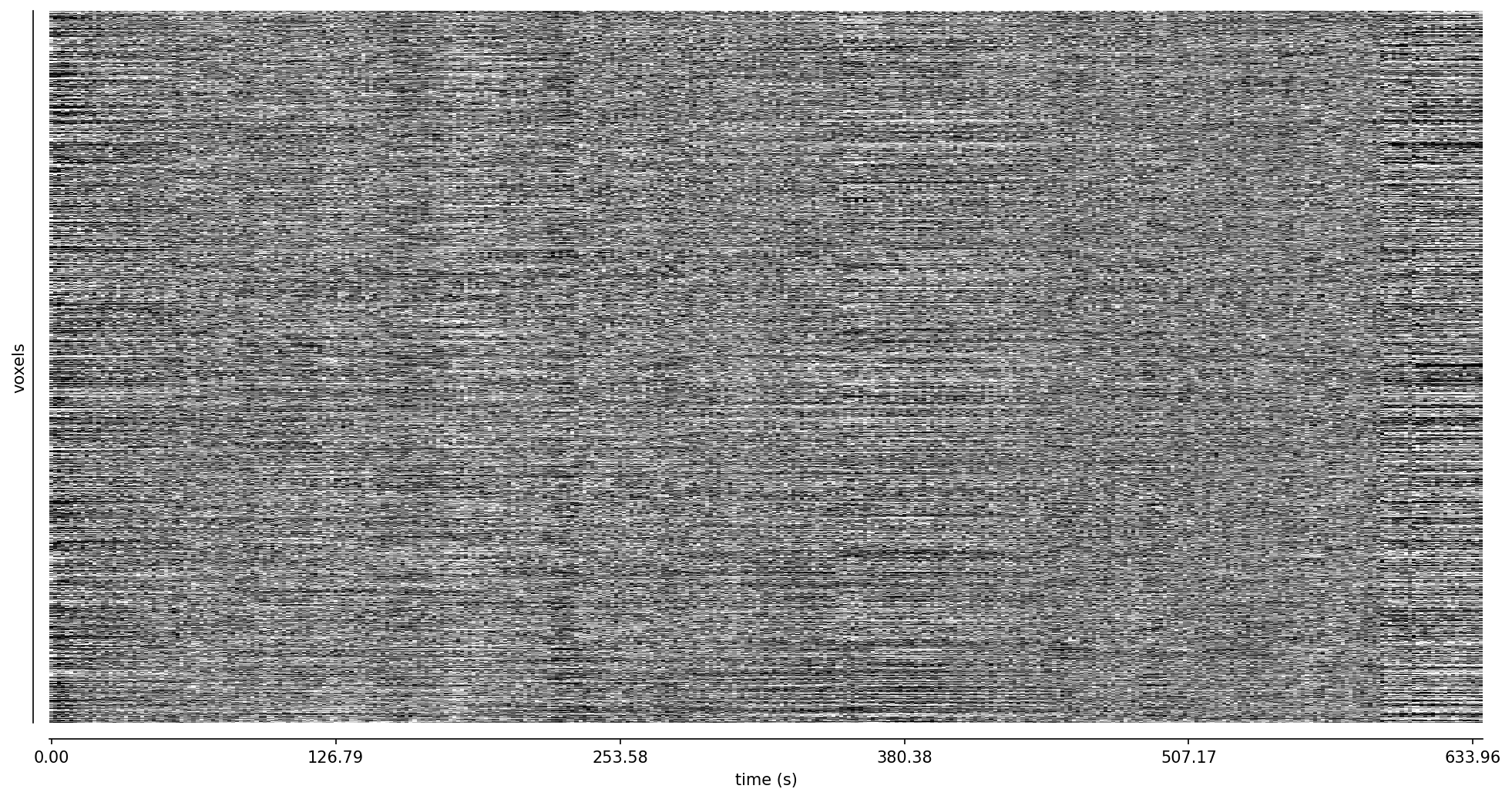
Fig. 34 Carpet plot of the optimally combined data.